I associate derivatives with practicing differentiation rules on increasingly implausible looking functions. If you have similar memories, you'll remember it's a mechanical, rather boring process. Boring for humans is good for computers though, because that means it's amenable to automation. So automate it we will, using a technique called Automatic Differentiation (AD). What's surprising about AD is that it generalizes so well: AD not only calculates the derivative of mathematical functions, but also of programs using constructs like conditionals, loops, recursion and higher-order functions. To highlight this, people have coined differentiable programming as an umbrella term for the various uses and applications AD enables.

AD has become a widely used technique, as it plays a pivotal role in deep learning. Gradient descent-based optimization - how the billions of weights in neural networks are trained - needs derivatives, and AD calculates them extremely efficiently. It's up to 6 or 7 orders of magnitude faster than naïve approaches. That's the difference between one day to train a model and 2,738 years! With the current explosion of interest in deep learning, AD is a hot research topic as well. That said, it has many other applications, notably computer graphics, and risk analysis in finance.

This post explains how AD works in-depth, both its forward and somewhat baffling reverse mode. It is aimed at programmers - I'll assume you remember some notions of what differentiation is and some rules, but will link to further information to explore at your leisure. Examples are in Rust, so some experience with typed, functional languages is helpful but not necessary. The implementation does not rely on Rust-specific features.

All code is on GitHub.

What are derivatives, really?

Derivatives are typically explained in visual terms using graphs of functions. For a scalar function ℝ→ℝ, the derivative at a particular point is represented by the tangent of the function at that point. This interpretation builds useful intuition, and I recommend 3blue1brown's excellent visual series if you're unfamiliar or need a refresher. The visual interpretation works for functions that are two or three dimensional - for example a function 𝑓:ℝ²→ℝ describes the height of an imagined terrain as a function of (x,y) coordinates. The derivative of such a function has two components, one for each input: ∂𝑓/∂𝑥 and ∂𝑓/∂𝑦. These are called the partial derivatives, and together describe the slope of the terrain at a particular (x,y) coordinate.

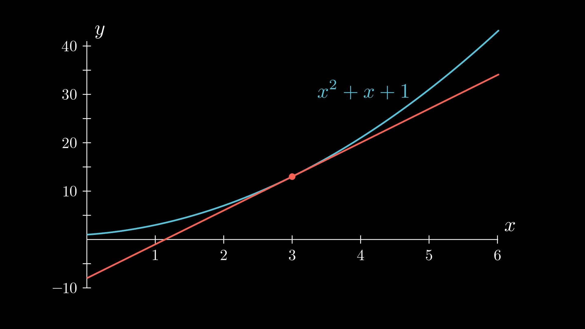
A tangent line at x=3

However, no one can imagine a four-dimensional space, let alone GPT-3's 175 billion-dimensional space of weights. To deal with that, another perspective is that the derivative is a measure of the sensitivity of a function to its inputs. (I'll use the terms inputs and outputs of functions rather than parameters or domain, because it's more familiar to programmers.)

This view is common in risk analysis. Say you have a function that, based on various observable values, calculates today's value of an investment. The observables could be interest rates, inflation rates, foreign exchange rates, anything that affects the value of the investment. To gauge how risky the investment is, we'd like to know how its value changes if the observables change. If the value of the investment changes significantly for a small change in say interest rate, then that indicates it is particularly sensitive to interest rates. If we don't like such a high exposure to interest rates, we may want to hedge this risk.

It turns out that the derivative is exactly a measure for the sensitivity of the output(s) of a function to each of its inputs. More accurately, for a function 𝑓: ℝ³→ℝ, i.e. a function with three inputs and one output, the derivative function 𝑑𝑓: ℝ³→ℝ³ has three partial derivatives at each input value. The partial derivative is a measure of how the value of 𝑓 changes, if the corresponding input value changes - in other words, how sensitive 𝑓 is to changes in the value of each of its inputs. What's neat about partial derivatives is that you can linearly combine them to get the sensitivity to several inputs as well (for well-behaved functions, at least). The partial derivatives are exactly the quantities you need to figure out everything there is to know about the sensitivity of the function to input changes.

But how is this measure interpreted and where does it break down? It turns out that the derivative is just an approximation. To be exact, the derivative is the best linear approximation of the function.

In practice linear approximations of non-linear functions are only good close to the point where they are evaluated. If our investment is worth $1000 today, at an interest rate of 1%, and sensitivity to interest rate is $10 per 0.01% at 1% interest rate, then a reasonable estimate of the value of the investment at 1.01% interest rate is $1010. However it is just an estimate, and the further away from the interest rate of 1%, the more inaccurate the estimate will be. The exception to this is if the function is itself linear - in that case a linear approximation is exact.

To change tack, having rid ourselves of the necessity to imagine 15-dimensional landscapes, we can now also understand how deep learning networks are trained through an optimization process called gradient descent. A neural network can be understood as a machine that has potentially billions of parameters, called weights, which need to be adjusted so that the machine produces the desired outputs. During training, we give the machine an input and it produces an output. We compute the error - the difference between the machine's output, and the desired output. We'd like to make this error as small as possible. Because the error is a function of the weights of the machine, we can calculate how sensitive the error is to small changes in each of the weights by calculating the partial derivative of the error function to all the (potentially billions) of weights. Once we know how the error changes with the weights, we can adjust the weights to make the error smaller - if the sensitivity is positive, we'll make that weight a bit smaller, if it's negative, we'll make it a bit bigger. Lather, rinse, repeat, and before you know it you can generate some amazing images.

What differentiable programming means

Let's start with a simple example - a function that takes and returns a single floating point number.

fn f(t: f64) -> f64 {
    t.powi(2) + t + 1.0
}

Let's say we're interested in having a function df which represents the derivative of f.

How can we figure out df from f automatically? Besides automatic differentiation, there are two other approaches: symbolic and numeric differentiation. I'll briefly discuss them to better understand what makes AD so effective.

Symbolic differentiation

An exhaustive set of rules exists to calculate df from f, so by applying these rules or asking something smarter than me, we can write df directly:

fn df_sym(t: f64) -> f64 {
    2.0 * t + 1.0
}

This approach is called symbolic differentiation. It's easy to do for this simple example, but with common programming constructs like shared variables, iteration, recursion and conditionals, it can be very hard to come up with an efficient closed formula for the derivative.

Numeric differentiation

An alternative is numeric approximation, which follows from the definition of derivative:

fn df_num(t: f64, h: f64) -> f64 {
    (f(t + h) - f(t)) / h
}

For some small number h. Numeric differentiation, while simple to implement, is not without problems: choosing an h that is just right, and doesn't lead to numerical instabilities is tricky. There are approaches that solve some of these problems, but simplicity is lost. Also this needs two evaluations of f, which is not ideal.

Comparing symbolic and numeric differentiation:

let t = 5.0;
println!("Symbolic: {}", df_sym(t));

let h = 0.000001;
println!("Numeric: {}", df_num(t, h))

Results in:

Symbolic: 11
Numeric: 11.000001002514637

Automatic differentiation

The idea of automatic differentiation is to compute the derivative at the same time as the function itself, by applying differentiation rules one operation at a time. Let's do that manually first.

We're aiming for a function f_ad(t_dual: (f64, f64)) -> (f64, f64). The argument t_dual is a tuple with the value of t as the first element, and its derivative as the second element. The combination of these two is typically called a dual number. We need t_dual to be a dual number because the input to f_ad might be the result of another automatically differentiated function. The result of f_ad is also a dual number: it returns the value f would normally compute, as well as its derivative.

Here's the implementation in AD style:

fn f_ad(t_dual: (f64, f64)) -> (f64, f64) {
    let (primalt, tangentt) = t_dual;
    let (primal0, tangent0) = (primalt.powi(2), 2.0 * primalt * tangentt);
    let (primal1, tangent1) = (primal0 + primalt, tangent0 + tangentt);
    let (primal2, tangent2) = (primal1 + 1.0, tangent1);
    (primal2, tangent2)
}

Each operation in the original f is on a separate line. On each line, the regular value, the primal, is updated, along with the tangent, which represents the derivative. The calculation of the tangent is the result of applying differentiation rules, most importantly the chain rule. It's worth dwelling on the the chain rule for a bit, because it's essential to AD.

The chain rule tells us how to calculate the derivative of function composition - a fancy name for passing the result of a function e into a function f, i.e. f(e(t)). This is written as 𝑓 ∘ 𝑒, where ∘ denotes function composition. (I used e here instead of the more typical g, because e comes before f). The chain rule is used when calculating tangent0.

The first component of tangent0 is 2.0 * primalt, because of the power rule. Then that's multiplied by tangentt because of the chain rule, which comes into play because t_dual may be the result of applying another function e. t_dual's tangent is the derivative of e(t). tangent0 then needs to determine the derivative of e(t).powi(2), in other words the composition of e and powi. Hence the chain rule tells us to derive powi, and then multiply that by the derivative of e, which is tangentt.

Note that calculating the primal at each step only needs previously calculated primal values - this seems obvious but is not true for the tangent, which needs both primal and previous tangent values. tangent0 for example uses the value 2.0 from its own primal, as well as primalt and tangentt.

Finally, here's how to call f_ad:

println!("Automatic: {}", f_ad((t, 1.0)).1);

Why is the initial tangent 1.0? Because that's the derivative of the identity function 𝑖𝑑(𝑥)=𝑥.

This outputs:

Automatic: 11

Have a go yourself at the Rust playground.

Towards automatic differentiation

The next sections develop a minimal implementation of AD. It proceeds in steps: first, we make the manual implementation of AD actually automatic. Then, we'll investigate the efficiency of the implementation, and iteratively improve it. Each step reveals an insight into how and why AD works.

Generally, AD can be implemented in two ways: source to source transformation, or via operator overloading. Source to source transformation analyses the source of the original program f and generates the code for f_ad. Depending on the constructs the transformation supports, it is entirely transparent to the programmer. However, it needs a lot of machinery for parsing and producing efficient code, which is not relevant to the core ideas of AD. I'll use operator overloading here, but the ideas are transferable.

Actually automatic through operator overloading

First let's refactor the tuples into a proper type of dual numbers: Dual. The idea is to define operators like sum and product on Dual using operator overloading, so that we can write programs that work with dual numbers as if we're dealing with floating point numbers. Except now functions compute the value and derivative at the same time! This process is somewhat similar to introducing a library for complex or rational numbers. Here's the type for dual numbers:

struct Dual {
    primal: f64,
    tangent: f64,
}

Primitive Dual values are constant and var:

impl Dual {
    fn constant(value: f64) -> Self {
        Dual {
            primal: value,
            tangent: 0.0,
        }
    }

    fn var(value: f64) -> Self {
        Dual {
            primal: value,
            tangent: 1.0,
        }
    }
}

Both constant and var have a user-defined primal value, and only differ in their derivative. constant represents the constant function f(x) = C. Constant functions have a derivative that's 0 everywhere. var represents the identity function f(x) = x, with a derivative that's 1 everywhere. (Why call it var and not id? Because typically it's used to define new variables we'd like to calculate the derivative of.)

Next is overloading addition and multiplication for Dual by using the sum and product rules in tangent:

// Add trait omitted
fn add(self, rhs: Self) -> Self::Output {
    Dual {
        primal: self.primal + rhs.primal,
        tangent: self.tangent + rhs.tangent,
    }
}

// Mul trait omitted
fn mul(self, rhs: Self) -> Self::Output {
    Dual {
        primal: self.primal * rhs.primal,
        tangent: rhs.tangent * self.primal + self.tangent * rhs.primal,
    }
}

And also define powi for Dual:

impl Dual {
    fn powi(self, exp: i32) -> Self {
        Dual {
            primal: self.primal.powi(exp),
            tangent: f64::from(exp) * self.primal.powi(exp - 1) * self.tangent,
        }
    }
}

The example function f now becomes:

fn f_ad_dual(t: Dual) -> Dual {
    t.powi(2) + t + Dual::constant(1.0)
}

// call site:
f_ad_dual(Dual::var(3.0))

It looks like the original function f, with a bit of syntactic noise. Some languages allow defining new literals, or implicit conversions, which allows getting rid of the call to Dual::constant. Another way to achieve that would be to define overloads for all operators for Dual and f64 in all possible combinations. In unityped languages with operator overloading, there isn't even be a type signature to change, so f may not need to change at all.

I'll be using graphs throughout this post to illustrate the calculation of the tangent, which is straightforward now but will become more involved. Here's a graph representing the calculation of df(3), i.e. calculation of Dual.tangent at t=3:

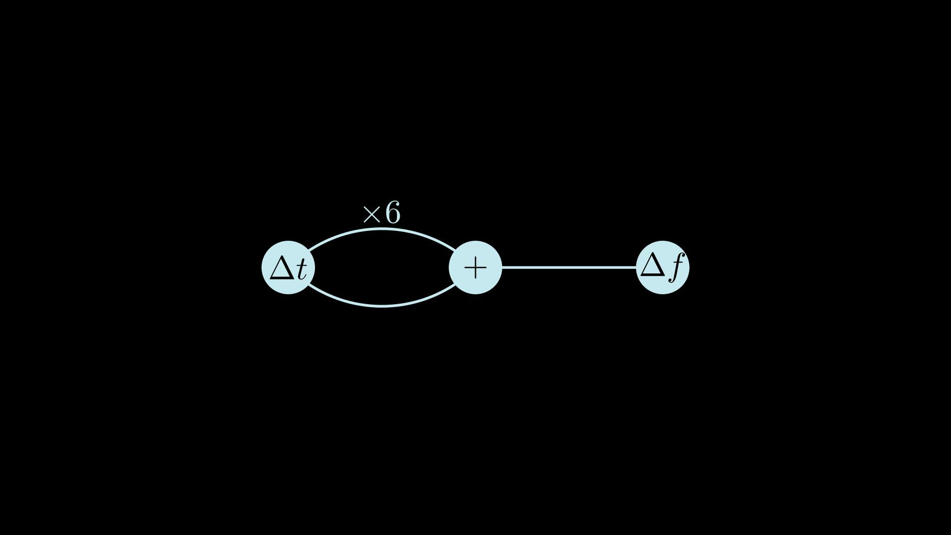
On the left is the tangent of the input t, shown as Δ𝑡. Edges scale the tangent with a factor, in this case because of the chain rule. If no factor appears on the edge, it is equal to one. At each + node, tangents are added.

Here's how the calculation proceeds - from left to right, a detail that will become important.

Intermezzo: Dual numbers

Mathematically, Dual numbers are expressions of the form a+bϵ where a and b are real numbers, and ϵ is a "small quantity" such that ϵ²=0. Think of complex numbers but ϵ instead of 𝑖.

What's interesting about dual numbers is that we can think of the first part of the dual number as the primal, and the second part as the derivative, and end up with rules for differentiation that are the same as the rules for symbolic differentiation. For sums and products this needs only simple arithmetic:

• Sum: (a+bϵ) + (c+dϵ) = (a+b) + (c+d)ϵ.

• Product: (a+bϵ)(c+dϵ) = ac + adϵ + bcϵ + bdϵ² = ac + (ad + bc)ϵ since ϵ²=0.

Compare this with the implementation of Dual for sum and product: the first part of the dual number corresponds to the primal, the second part to the tangent. A chain rule with a similar shape can be derived as well.

Generalizing dual numbers

We left the previous section with a Dual type that consists of two floating point numbers. However, the derivative of a function with multiple inputs has multiple components: the partial derivative with respect to each input. This means that a single float may not be enough for the tangent field. To address that, let's refactor Dual. At this point some of this might seem abstraction for the sake of abstraction, but it will come in handy later.

First redefine Dual as follows:

struct Dual<T> {
    primal: f64,
    tangent: T,
}

The primal is still a f64 value, but tangent is left generic. We can recover our old Dual by instantiating T as f64, so this is strictly a generalization. However, just any T won't do - we must be able to apply differentiation rules to it.

It turns out that to calculate derivatives, T only needs a zero element, an addition and scale operation - which corresponds to T forming a vector space. I don't know how to explain intuitively why this is true! But you can check the differentiation rules to see that it is. An accurate statement and proof can be found on the Linearity of differentiation Wikipedia page.

Anyway, trusting the math hasn't failed me yet, so we can represent this requirement on T by a Rust trait:

trait VectorSpace {
    fn zero() -> Self;
    fn add(&self, rhs: &Self) -> Self;
    fn scale(&self, factor: f64) -> Self;
}

And implement VectorSpace for floats:

impl VectorSpace for f64 {
    fn zero() -> Self {
        0.0
    }

    fn add(&self, rhs: &Self) -> Self {
        self + rhs
    }

    fn scale(&self, factor: f64) -> Self {
        self * factor
    }
}

Now we can overload operators on Dual<T> for any T which is a VectorSpace:

impl<T: VectorSpace> Dual<T> {
    fn constant(primal: f64) -> Self {
        Dual {
            primal,
            tangent: T::zero(),
        }
    }

    fn add_impl(&self, rhs: &Dual<T>) -> Dual<T> {
        Dual::new(self.primal + rhs.primal, self.tangent.add(&rhs.tangent))
    }

    fn mul_impl(&self, rhs: &Dual<T>) -> Dual<T> {
        Dual::new(
            self.primal * rhs.primal,
            rhs.tangent
                .scale(self.primal)
                .add(&self.tangent.scale(rhs.primal)),
        )
    }
}

I'm omitting the ceremonial implementations of the Add and Mul traits. It's now possible to write f with our new Dual<T> type:

fn f<T: VectorSpace>(x: &Dual<T>) -> Dual<T> {
    t.powi(2) + t + Dual::constant(1.0)
}

fn df(t: f64) -> f64 {
    let res = f(&Dual::new(t, 1.0));
    res.tangent
}

Dual<T> can now be used like Dual could, and we seem to be back where we started. We have gained some power though - let's actually leverage it next.

Forward mode and Reverse mode

AD comes in two flavours, called modes: forward mode and reverse mode. These two modes can also be mixed. So far we've implemented forward mode, which is the easiest to understand. It's called forward mode because the computation of the derivative flows in the same "forward direction" as the evaluation of the main program. In reverse mode, part of the calculation will happen in the opposite direction - we'll build up to how exactly that works. For the moment, let's consider our current implementation more in depth, to understand what its limits are.

For functions that have a single input, but many outputs, forward mode works efficiently. More concretely, calculating the derivative only adds a constant factor overhead to each operation - a few more additions and multiplications. Here's an example of a function with multiple outputs, and how we can get its derivatives:

fn f_2out<T: VectorSpace>(x: &Dual<T>) -> (Dual<T>, Dual<T>) {
    let ref y = x.sin() * x.sin();
    (y + x * Dual::constant(10.0), x + y * Dual::constant(20.0))
}

fn df_2out<T: VectorSpace>(x: f64) -> (f64, f64) {
    let (dx1, dx2) = f_2out(&Dual::new(x, 1.0));
    (dx1.tangent, dx2.tangent)
}

df_2out returns the derivative of each of its outputs with respect to x, and needed just one call to f_2out to achieve that. There are two derivative values now, but forward mode AD can calculate both of them with a constant factor overhead.

This is great news, however a function with multiple inputs tells a different story.

fn f<T: VectorSpace>(x: &Dual<T>, y: &Dual<T>) -> Dual<T> {
    x * y
}

fn df_v1(x: f64, y: f64) -> (f64, f64) {
    (
        f(&Dual::new(x, 1.0), &Dual::constant(y)).tangent,
        f(&Dual::constant(x), &Dual::new(y, 1.0)).tangent,
    )
}

Because we need to calculate the partial derivative to each of the two inputs separately, we need two calls to f. This is bad for efficiency: for gradient optimization problems in deep learning with billions of inputs, we'd need billions of calls to the function! This approach will certainly not do.

Let's visualize what's going on. Here's a graph representing the calculation of the derivative of df(3, 2), i.e. calculation of Dual.tangent at x=3 and y=2:

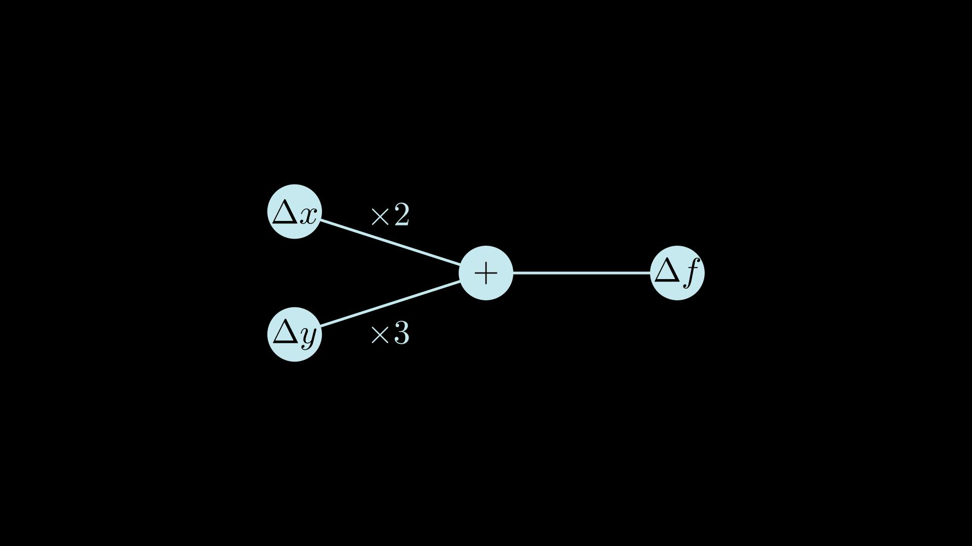
On the left are the tangents of x and y, shown as Δ𝑥 and Δ𝑦. The factors on the edges from Δ𝑥 and Δ𝑦 are because of the product rule: (𝑥𝑦)′ = 𝑥𝑦′ + 𝑦𝑥′. This shows visually why we had to evaluate twice, once with Δ𝑥=1 and once with Δ𝑦=1: a single evaluation of f with both Δ𝑥=1 and Δ𝑦=1 would give the total derivative. The total derivative is the sensitivity of the function when all its inputs change at once; but we're not interested in that. We need the partial derivatives, so we get the sensitivity to each input individually.

First fix: many calls to one call

If you've ever dealt with a function that has significant overhead on each call - say, it accesses a database - then you'll have learnt that it's not a good idea to call that function multiple times in a loop. It's much better to pass all the inputs at once, and re-implement the function to deal with multiple values more efficiently by accessing the database just once.

We can apply a similar idea here. We're calling f multiple times, each time with different tangent values. Instead we can make the tangent T an array, to pass them all at once into a single call.

This is where the Dual<T> abstraction pays off. No need to change the Dual type - just implement VectorSpace for arrays:

impl<T: Copy + VectorSpace, const N: usize> VectorSpace for [T; N] {
    fn zero() -> Self {
        [T::zero(); N]
    }

    fn add(&self, rhs: &Self) -> Self {
        let mut result = [T::zero(); N];
        for (i, (l, r)) in self.iter().zip(rhs).enumerate() {
            result[i] = l.add(r);
        }
        result
    }

    fn scale(&self, factor: f64) -> Self {
        let mut result = [T::zero(); N];
        for (i, v) in self.iter().enumerate() {
            result[i] = v.scale(factor);
        }
        result
    }
}

Arrays are added element by element (point-wise), and scaling applies to each element.

Keeping f the same, but changing df:

fn df_v2(x: f64, y: f64) -> [f64; 2] {
    f(&Dual::new(x, [1.0, 0.0]), &Dual::new(y, [0.0, 1.0])).tangent
}

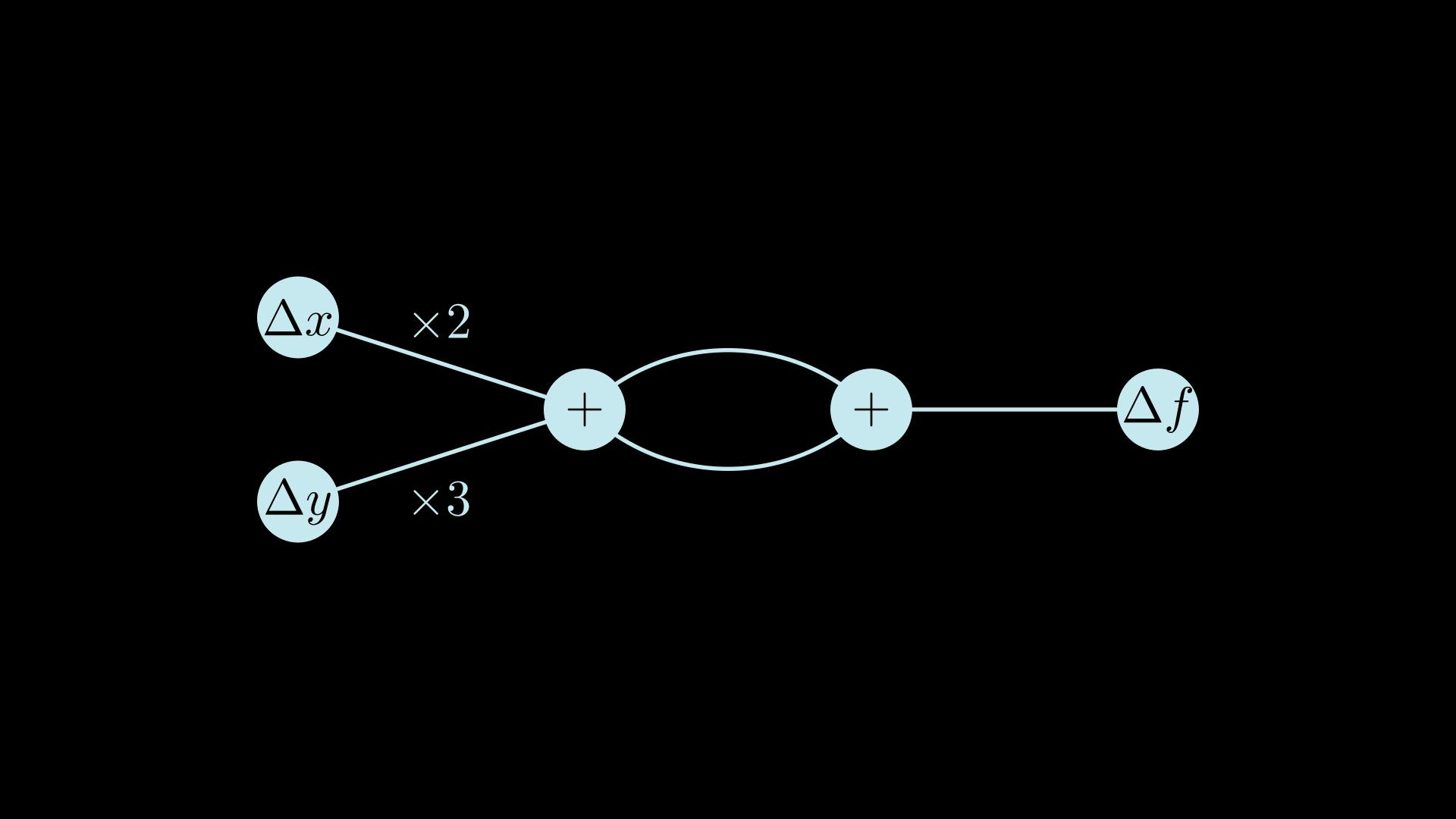
This works out better: the function is only called once. The following animation visualizes the computation now:

Evaluation still proceeds forwards through the graph, as before. The array representation allows us to evaluate the function only once, and still get all the partial derivatives.

Alas: memory usage for the arrays is quadratic in the number of inputs! That's workable for a low number of inputs, but is intractable for billions.

Second fix: introduce an intermediate representation

Those arrays certainly look sparse. Perhaps a sparse encoding is a way forward? Unfortunately, that won't work, because as the computation proceeds they don't remain sparse for long, as the visualization shows. Instead, let's use a related idea, and replace the arrays with an intermediate representation. This splits the calculation in two passes: the first builds an intermediate representation, the second uses the intermediate representation to compute the derivatives.

For the intermediate representation, we introduce a new Delta type:

enum Delta {
    Zero,
    Var(usize),
    Scale(f64, Rc<Delta>),
    Add(Rc<Delta>, Rc<Delta>),
}

If you're not familiar with Rust: Delta is a union type with four possible cases. Rc is a reference counted smart pointer - for this post it's safe to just squint and pretend the Rcs are not there.

Delta is a reified representation of VectorSpace operations - and captures the structure of the derivative computation as a directed acyclic graph. Var represents an input variable like x or y; the argument is a unique number to identify the variable.

To use Dual<Delta>, we need to make Delta a VectorSpace:

impl VectorSpace for Rc<Delta> {
    fn zero() -> Self {
        Rc::new(Delta::Zero)
    }

    fn add(&self, rhs: &Self) -> Self {
        Rc::new(Delta::Add(Rc::clone(self), Rc::clone(rhs)))
    }

    fn scale(&self, factor: f64) -> Self {
        Rc::new(Delta::Scale(factor, Rc::clone(self)))
    }
}

The last piece of the puzzle is evaluating the intermediate representation to the partial derivatives.

pub fn eval_delta(scale_acc: f64, delta: &Delta, result: &mut Vec<f64>) {
    match *delta {
        Delta::Zero => (),
        Delta::Var(i) => result[i] += scale_acc,
        Delta::Scale(factor, ref d2) => eval_delta(scale_acc * factor, d2, result),
        Delta::Add(ref l, ref r) => {
            eval_delta(scale_acc, l, result);
            eval_delta(scale_acc, r, result);
        }
    }
}

eval_delta is memory-efficient: it updates a single array in place. It iterates depth-first through the graph described by Delta, and accumulates scale factors along each path from the root to the Var or Zero leaves. When it encounters a Var case, which is necessarily a leaf, it just adds the accumulated scale factor to the right place in the result array.

Putting all of that together, the third version of df becomes:

fn df_v3(x: f64, y: f64) -> Vec<f64> {
    let dual_delta = f(
        &Dual::new(x, Rc::new(Delta::Var(0))),
        &Dual::new(y, Rc::new(Delta::Var(1))),
    );
    let mut result = vec![0.0, 0.0];
    eval_delta(1.0, &dual_delta.tangent, &mut result);
    result
}

This looks much better! The first pass, executing f, returns a Delta intermediate representation, and then in a second pass, eval_delta accumulates the scale factors "in reverse" with respect to the usual evaluation order of the program. This reversal is visible as the scale_acc parameter of eval_delta. The evaluation process can be visualized as follows, as before for df(3,2). Note that we now have an explicit representation of this graph as a result of the forward pass, for this example Add(Scale(2.0, Var(0)), Scale(3.0, Var(1))).

In other words, this is a "beta version" of reverse mode AD - there is still an ingredient missing, as we'll see - but it explains where the name comes from. Using a single depth-first traversal of the Delta graph, it's possible to get the partial derivatives with respect to all the inputs in one reverse sweep. And importantly, we don't need an amount of memory that's the square of the number of inputs anymore.

Finally efficient: dealing with sharing

Now there is one remaining problem - if the original program contains shared variables, eval_delta does too much work. Here's a problematic example:

fn f_sharing_bad<T: VectorSpace>(x: &Dual<T>, y: &Dual<T>) -> Dual<T> {
    let ref s = x * y;
    s + s
}

The s variable is used twice in the final result, and as expected the primal of s is only calculated once and then reused in the addition. But, the calculation of the tangent of s is done twice in eval_delta. Here's the Delta graph for x=3 and y=2:

We want our derived program to have asymptotically the same complexity as the main program, and not respecting sharing can easily blow up the complexity.

This smells like a dynamic programming problem: parts of the graph are shared, but they're being evaluated repeatedly. To achieve the same asymptotic performance as the main program, we have to make sure that each node in the Delta graph is evaluated only once. As usual in dynamic programming, part of the answer is memoization: as we calculate scale factors, we'll need to store for each node what the factor is up to that point. To guarantee we visit every node only once, and we have accumulated the necessary factors, we have to visit the graph in reverse topological order. Luckily, we already have such an order: it's just the reverse order of the forward pass!

To accomplish all this, we need to make two changes:

1. Introduce a Trace type to record the evaluation order of the operations in the forward pass; and

2. Use Delta::Var to represent intermediate variables explicitly. Since we can't detect which variables are shared and which ones are not, we assign the result of each operation to a temporary Var in the trace. Put another way, each node in the graph is represented by a Var.

Here's the salient parts of the implementation. First, the Trace type.

struct Trace {
    trace: RefCell<Vec<Rc<Delta>>>,
}

Ignoring the RefCell and Rc, this is just a resizable array (Vec in Rust) of Delta values. We're going to treat this Trace as a stack: in the forward sweep, each tangent operation gets pushed on it, and in the reverse sweep, we'll be popping operations to calculate derivatives. The stack ensures we are visiting each node just once and in reverse topological order.

Then the Dual type needs to be augmented with a Trace, so we can record each operation in it:

struct DualTrace<'a> {
    trace: &'a Trace,
    dual: Dual<Rc<Delta>>,
}

This means we need to redo the addition and multiplication overloads we did earlier for DualTrace. For each operation we can delegate to the overload for Dual, but need to do two extra things:

1. Push the operation on the Trace;

2. Return a new Var to represent this operation. This intermediate variable will then used to store and share the result, so it is only evaluated once.

Remember way back in the introduction, we rewrote f to look like this:

fn f_ad(t_dual: (f64, f64)) -> (f64, f64) {
    let (primalt, tangentt) = t_dual;
    let (primal0, tangent0) = (primalt.powi(2), 2.0 * primalt * tangentt);
    let (primal1, tangent1) = (primal0 + primalt, tangent0 + tangentt);
    let (primal2, tangent2) = (primal1 + 1.0, tangent1);
    (primal2, tangent2)
}

That's very similar to how we're using Var now: each operation becomes an implicit let Var_i = Add(...) in the trace.

Here's what that looks like for addition:

impl Trace {
    fn push(&self, op: Dual<Rc<Delta>>) -> Dual<Rc<Delta>> {
        let mut trace = self.trace.borrow_mut();
        let var = Dual {
            primal: op.primal,
            tangent: Rc::new(Delta::Var(trace.len())),
        };
        trace.push(op.tangent);
        var
    }
}

Trace.push adds a new operation (Scale, Add or Zero) to the end of the trace, and returns a new Delta::Var to represent the result of that operation. Now addition:

impl<'a> DualTrace<'a> {

    fn delta_push(&self, op: Dual<Rc<Delta>>) -> DualTrace<'a> {
        let dual = self.trace.push(op);
        DualTrace {
            trace: self.trace,
            dual,
        }
    }

    fn add_impl(&self, rhs: &DualTrace<'a>) -> DualTrace<'a> {
        let op = &self.dual + &rhs.dual;
        self.delta_push(op)
    }
}

And the same for other operations. This maintains the invariant that the result of any operation always has a Var as tangent. We'll leverage this fact when doing the reverse sweep, as it allows us to detect sharing explicitly.

Here's the latest and greatest eval. It uses eval_delta which is unchanged from before.

pub fn eval(inputs: usize, dual_trace: &DualTrace) -> Vec<f64> {
    let mut result = vec![0.0; dual_trace.trace_len()];
    let mut trace = dual_trace.trace_mut();

    eval_delta(1.0, &dual_trace.dual.tangent, &mut result);

    while trace.len() > inputs {
        let deltavar = trace.pop().unwrap();
        let idx = trace.len();
        if result[idx] != 0.0 {
            eval_delta(result.pop().unwrap(), &deltavar, &mut result);
        }
    }
    result
}

Let's see how to use all this, then dig into some details.

fn f_sharing_fixed<'a>(x: &DualTrace<'a>, y: &DualTrace<'a>) -> DualTrace<'a> {
    let ref s = x * y;
    s + s
}

fn df_sharing_fixed(x: f64, y: f64) -> Vec<f64> {
    let trace = Trace::new();
    let x = &trace.var(x);
    let y = &trace.var(y);
    let dual_trace = f_sharing_fixed(x, y);
    eval(2, &dual_trace)
}

For this example with x=3 and y=2, the trace after the forward pass is an array of 5 elements:

[ Var 0, // x
  Var 1, // y
  Add(Scale(2.0, Var 0), Scale(3.0, Var 1)), //let s = 2x + 3y
  Add(Var 2, Var 2) // let r = s + s
  Var 3 ] // r

(I've omitted some parentheses to make it easier to read)

The trace makes sharing explicit. Each Var's id is a valid index in the array, which refers to where that "variable" is defined. In eval, a result array is allocated for each element of the trace, and this array is where the derivative for the corresponding variable is accumulated. The trace is also used to make sure each node is visited only once. Here eval's reverse sweep is animated, always for x=3 and y=2. The result array is shown at the top.

And there you have it! From forward to efficient, reverse mode AD in four steps.

If you read this far, you may as well consider subscribing to my newsletter, and/or follow me on Twitter.

Acknowledgements and further references

The main inspiration and origin of this post is the paper "Provably Correct, Asymptotically Efficient, Higher-Order Reverse-Mode Automatic Differentiation" by Faustyna Krawiec, Neel Krishnaswami, Simon Peyton Jones, Tom Ellis, Andrew Fitzgibbon, and Richard Eisenberg, along with Simon Peyton Jones' presentation at Haskell Exchange 2021. You can find paper and presentation here.

Conal Elliot's papers were also very helpful and influential: Beautiful differentiation and The simple essence of automatic differentiation.

It helps having things explained from different perspectives. Here are a few other good links on the topic:

• Calculus on Computational Graphs: Backpropagation by Christopher Olah has more of a deep learning focus.

• Differentiable Programming from Scratch by Max Slater has a more mathematical focus, has inline JavaScript graphs you can play with, and shows how AD is used to de-blur images.

Any errors and omissions are entirely my responsibility.